
Anisotropic modeling and estimation for a two-dimensional semi-variogram based on the linear GSI Model: Taking DEM data as an example
Received date: 2019-09-12
Request revised date: 2020-03-11
Online published: 2021-01-19
Copyright
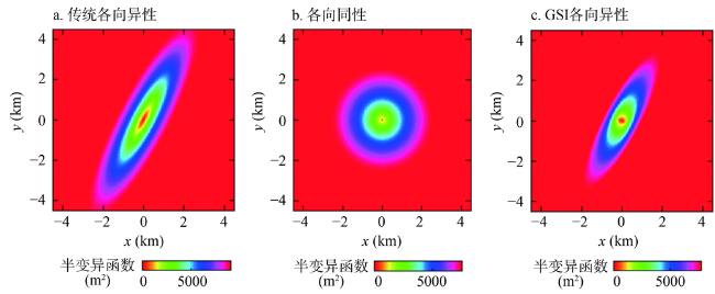
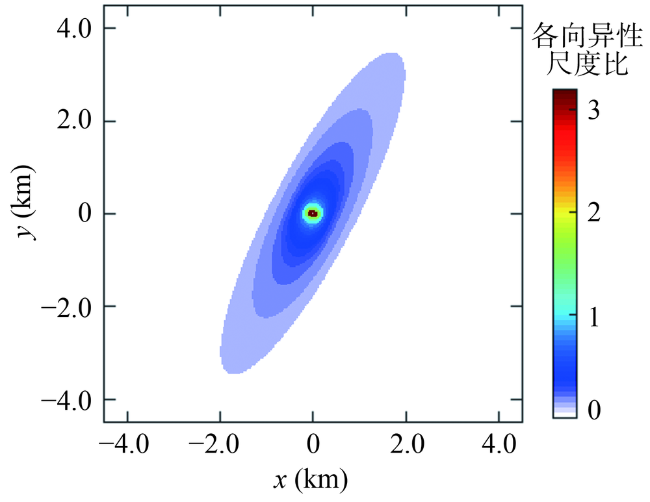
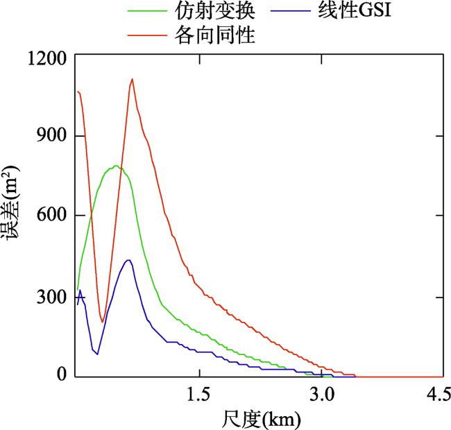
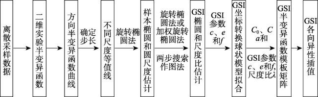
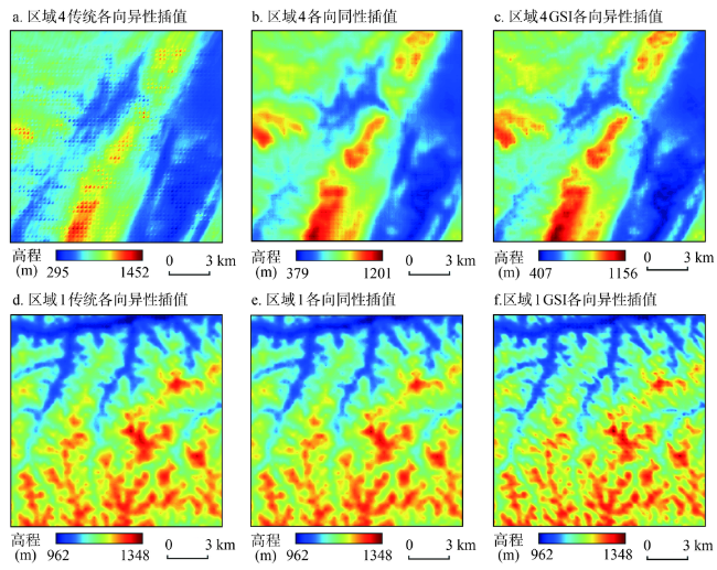
Anisotropy has been found to widely exist in the nature, and also regarded as one of the several essential attributes of geographical phenomena and processes. Therefore, it needs some complex models and methods to analyze and explain these phenomena, and deal with such problems as the optimization and interpolation for discrete monitoring points, or the uncertainty analysis by stochastic simulation over the space for some regional variables. The traditional treatment on an anisotropic modeling in kriging interpolation based on coordinate transformation does not fully consider or cannot accurately describe the internal structures of a two-dimensional anisotropic semi-variogram. Therefore, this study introduced a model named as linear generalized scale invariance (GSI) to simulate the anisotropic information of a 2D semi-variogram by using DEM as input data, while the system parameters were estimated by using the rotating ellipse and two-step search mapping method, and the comparisons of the two methods including GSI and traditional coordinate transformation applied in the fittings to the spherical model and the corresponding kriging interpolation were also made. The results firstly showed that anisotropy is common and ubiquitous in the spatial variability for topographic data, and the complexity is characterized by a change for an anisotropic ration when the corresponding scale changes, i.e. the different deformation behaviors over the whole semi-variogram maintained. However, some evidences showed that there are some regular features like an isotropic component existing in the anisotropic mechanism, such as a circular scale or circular contour. When facing such a complex structure, simple and rough treatment is obviously not enough. Secondly, the related parameters in GSI model can be estimated with high accuracy, such as the values of R2, which are all almost over 0.99 for the six regions. This indirectly proved that the validity and applicability of GSI model in the treatment to the anisotropic structure. In addition, for the fittings of the theoretical spherical model, the GSI model showed huge advantage over the traditional transformation and isotropic methods. Finally, as the enhanced effect originated from application of the GSI model in the interpolation processes, the coordinate transformation based on the linear GSI model had better improvement in accuracy than the traditional coordinate transformation, as well as a high ability of edge information recovery, although it exhibited some limitations and instability due to its complex covariance structure.
GAO Xin . Anisotropic modeling and estimation for a two-dimensional semi-variogram based on the linear GSI Model: Taking DEM data as an example[J]. GEOGRAPHICAL RESEARCH, 2020 , 39(11) : 2607 -2625 . DOI: 10.11821/dlyj020190794
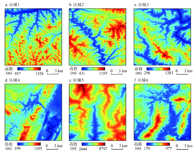
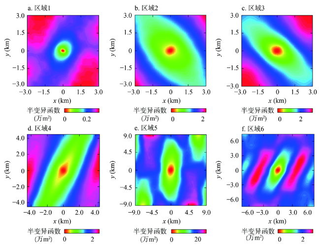
表1 研究区域的位置和地形地貌特征Tab. 1 The locations and terrain features of the six study regions |
| 研究区域 | 位置 | 所属山系 | 经纬度 |
|---|---|---|---|
| 区域1 | 陕西省北部 | 黄土高原丘陵沟壑区 | 37°N 109°E |
| 区域2 | 陕西省和湖北省交界处 | 秦岭山地 | 33°N 110°E |
| 区域3 | 陕西省和重庆市交界处 | 西北-东南走向的大巴山地 | 32°N 108°E |
| 区域4 | 湖北省和湖南省交界处 | 东北-西南延伸的武陵山地 | 29°N 108°E |
| 区域5 | 云南省北部 | 青藏高原横断山地 | 28°N 98°E |
| 区域6 | 福建省西南部 | 武夷山地 | 26°N 117°E |
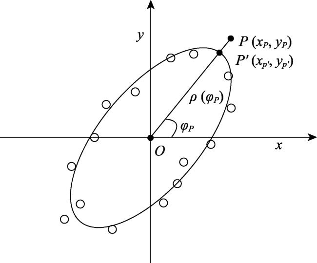
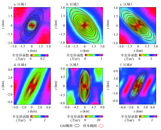
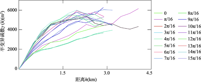
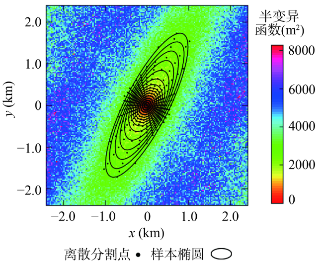
图8 区域1样本椭圆拟合结果Fig. 8 A fitting to the semi-variogram of region 1by using the rotating ellipse method |
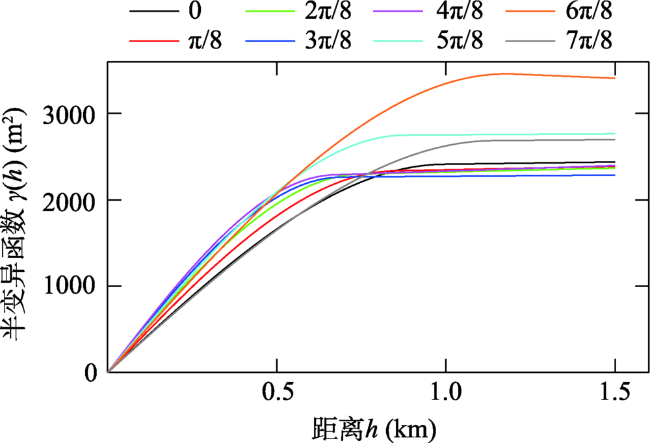
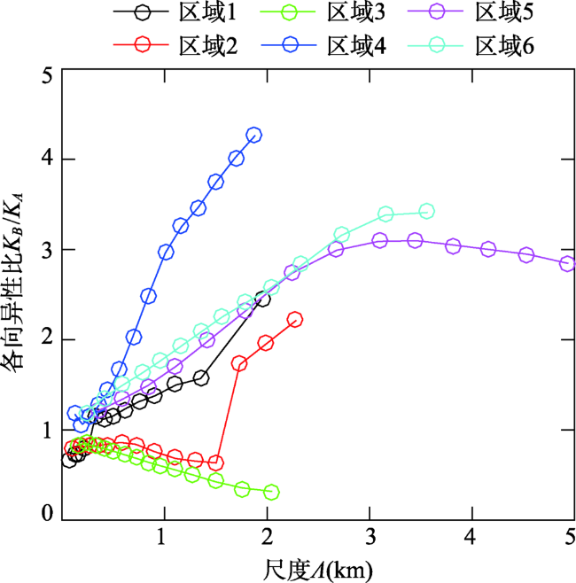
图9 六个区域各向异性比随尺度的变化Fig. 9 Anisotropic ratios corresponding to the scales of DEM data of the six regions |
表2 六个区域GSI模型相关参数估计结果Tab. 2 The estimates of the related parameters in the GSI model for the six regions |
| 研究数据 | 最小基台(m2) | 最大变程(m) | 圆尺度(m) | c | e | f | Rc2 | Re2 | Rf2 |
|---|---|---|---|---|---|---|---|---|---|
| 区域1 | 1556 | 678.61 | 410.37 | -0.1972 | -0.1696 | 0.1924 | 0.9987 | 0.9999 | 0.9968 |
| 区域2 | 6234 | 1093.35 | 572.31 | 0.1011 | -0.4123 | -0.2226 | 0.9997 | 1.0000 | 0.9996 |
| 923.18 | 0.2017 | -0.8014 | -0.4199 | 0.9991 | 0.9997 | 0.9990 | |||
| 区域3 | 13678 | 2122.37 | 232.70 | 0.1172 | -0.2011 | -0.2056 | 0.9956 | 0.9987 | 0.9885 |
| 区域4 | 4197 | 1261.67 | 199.14 | -0.2703 | -0.1836 | 0.1915 | 0.9907 | 0.9986 | 0.9927 |
| 区域5 | 79592 | 4213.85 | 29.48 | -0.0029 | -0.3980 | -0.1945 | 0.9995 | 0.9993 | 1.0000 |
| 区域6 | 15001 | 4423.97 | 49.58 | -0.1761 | -0.4026 | -0.0979 | 1.0000 | 0.9991 | 0.9981 |
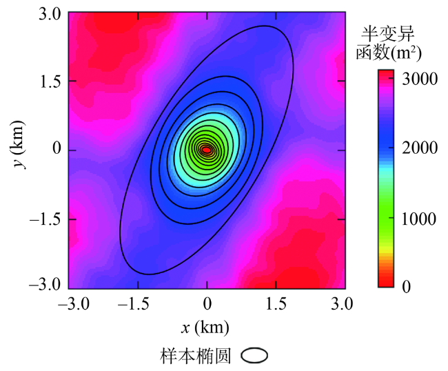
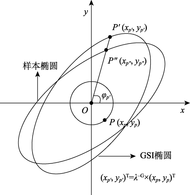
图10 GSI模型对样本椭圆拟合Fig. 10 A diagram showing the fitting of the GSI model to the previous fitted ellipse |
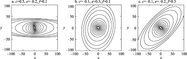
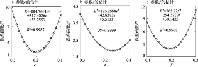
图11 基于二阶多项式对区域1半变异函数c、e和f的估计Fig. 11 The estimates of c, e and f of region 1 based on second-order polynomials |
表3 六区域传统各向异性、各向同性和GSI克里金估计均方根误差的均值和标准差Tab. 3 The means and standard deviations of RMSE concerned with kriging estimates versus the real values by using the traditional anisotropic, isotropic and GSI methods for the six regions |
| 均值(m) | 标准差(m) | ||||||
|---|---|---|---|---|---|---|---|
| 传统各向异性 | 各向同性 | GSI | 传统各向异性 | 各向同性 | GSI | ||
| 区域1 | 21.6778 | 22.1308 | 21.1273 | 0.1592 | 0.1546 | 0.1852 | |
| 区域2 | 30.5789 | 28.7977 | 28.1073 | 0.2777 | 0.2901 | 0.3217 | |
| 区域3 | 42.3000 | 28.5649 | 35.9589 | 0.2304 | 0.3804 | 0.2535 | |
| 区域4 | 59.4448 | 28.4447 | 23.2694 | 0.2821 | 0.1654 | 0.3421 | |
| 区域5 | 104.3453 | 42.1847 | 56.1315 | 1.0085 | 0.6435 | 0.5204 | |
| 区域6 | 31.9274 | 20.0796 | 23.7915 | 0.2454 | 0.2706 | 0.1671 | |
真诚感谢二位匿名评审专家在论文评审中所付出的时间和精力,评审专家针对本文内容和结构提出了许多建设性的意见,使本文获益匪浅。
| [1] |
冯波, 陈明涛, 岳冬冬, 等. 基于两种插值算法的三维地质建模对比. 吉林大学学报(地球科学版), 2019,49(4):1200-1208.
[
|
| [2] |
吕海洋, 盛业华, 李佳, 等. 基于RASM的紧支撑径向基函数自适应并行地形插值方法. 武汉大学学报(信息科学版), 2017,42(9):1316-1322.
[
|
| [3] |
聂磊, 舒红, 刘艳. 复杂地形地区月平均气温(混合)地理加权回归克里格插值. 武汉大学学报(信息科学版), 2018,43(10):1553-1559.
[
|
| [4] |
夏伟杰, 周建江, 姚楠. 各向异性的分形地形生成方法研究. 中国图象图形学报, 2009,14(11):2356-2361.
[
|
| [5] |
|
| [6] |
|
| [7] |
|
| [8] |
|
| [9] |
|
| [10] |
|
| [11] |
|
| [12] |
|
| [13] |
|
| [14] |
|
| [15] |
|
| [16] |
|
| [17] |
|
| [18] |
|
| [19] |
|
| [20] |
|
| [21] |
|
| [22] |
|
| [23] |
|
| [24] |
|
| [25] |
|
| [26] |
|
| [27] |
|
| [28] |
|
/
| 〈 |
|
〉 |