
高速铁路与出行成本影响下的全国陆路可达性分析
作者简介:蒋海兵(1978- ),男,江苏建湖人,博士,研究方向为城市和区域发展。E-mail: jianghb@igsnrr.ac.cn
收稿日期: 2014-12-23
要求修回日期: 2015-03-20
网络出版日期: 2015-07-12
基金资助
国家自然科学基金项目(41230632,41301108)
国家社会科学基金项目(14BSH036)
教育部人文社会科学研究项目(11YJC790077)
The land accessibility influenced by China's high-speed rail network and travel cost
Received date: 2014-12-23
Request revised date: 2015-03-20
Online published: 2015-07-12
Copyright
基于GIS技术与网络分析模型,应用可达性指数与标准交通经济成本参数(GTC),测度2020年规划高铁通车前后全国陆路可达性的空间格局与变化,探究高速铁路与出行成本影响下陆路可达性的特征。结果显示:从时间可达性看,高铁提高全国陆路可达性的整体水平与交通网络的客流运输效率,优化陆路交通网络,使跨区域中心城市之间联系日趋紧密,扩大中心城市的辐射范围,沿线重要城市人口覆盖范围急剧增长。高铁沿线站点、重要城市化地区与部分边远地区城市可达性获益最多,高铁对城市间中远距离关系影响突出,短距离影响主要局限于高铁沿线地区。此外,地区之间交通公平性差距结论并不统一。从经济可达性看,高铁对不同收入群体陆路可达性影响效果不同,对中低收入群体经济可达性影响有限,而对于高收入群体,随着旅行时间价值提高,经济可达性空间格局将不断接近时间可达性空间格局。
蒋海兵 , 张文忠 , 祁毅 , 蒋金亮 . 高速铁路与出行成本影响下的全国陆路可达性分析[J]. 地理研究, 2015 , 34(6) : 1015 -1028 . DOI: 10.11821/dlyj201506002
In China, with the drastic development of Chinese high-speed rail (HSR), assessing the impacts of HSR projects on transportation accessibility has recently been a hot topic for planners and researchers. Nevertheless, so far there has been limited research on exploring the implications of HSR on transportation accessibility, especially from the economic cost perspective. This paper studied the pattern and characteristics of land transportation accessibility influenced by China's HSR and travel cost. With the support of GIS technology and massive spatial data, the study constructed spatial analysis models based on shortest path algorithm and network analysis to calculate the accessibility index and generalized travel cost (GTC) parameter, so as to compare the pattern of land transportation accessibility before and after the construction of high speed rail for the planning year 2020. Firstly four accessibility indicators namely location indicator, economic potential, daily accessibility indicator and isochrones were used to measure time accessibility spatial distribution. Secondly, cost accessibility was measured by GTC. The accessibility maps address both the possible benefits and their spatial distribution. At last, the coefficient of variation of the accessibility values and its change before and after the construction of HSR was measured to represent the transport equity. Also the paper estimated whether the disparities of land accessibility were increased after the implementation of HSR. The results showed that from travel time perspective, HSR has improved overall level of the national land time accessibility and efficiency of passenger transportation, optimized the land transport network, then it tightened the connection among different metropolitan areas, expanded the radiation scope of the central cities. In addition HSR contributed to enlarging their service market demarcation and broadened markets of main central cities along the lines in short time distances. Furthermore cities along the HSR lines and in remote regions benefit most from the construction. HSR line had significant effect on the medium- and long-distance travel toward passengers, while short-distance travel mainly influenced the area along the railway lines.However, HSR led to more polarized accessibility patterns which indicated that various regions obtain unbalanced accessibility gain from HSR and enlarged the traffic inequity between different regions.As far as the travel cost accessibility was concerned, different demographic groups benefited differently from the HSR. Obviously travel cost accessibility pattern of the high-income groups was similar to the time accessibility pattern. On the contrary, for medium- and low-income groups, the HSR will not dramatically change the spatial pattern of economic accessibility. Therefore from traffic supply perspective, HSR only provided the possibility for the realization of the time-space convergence, which could greatly enhance regional social economic ties and reconstruct regional spatial pattern, which could not be achieved without passengers travel behavior' response to the HSR.
Key words: high-speed rail; accessibility; equity; spatial pattern
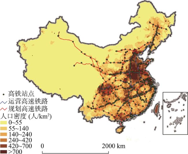
Fig. 1 The planning map of national high speed railway network of China in 2020图1 2020年全国高铁规划网络图 |
Tab. 1 The travel time variation between main cities without and with HSR in 2020表1 2020年高铁通车高铁通车前后全国中心城市之间的旅行时间变化 |
| 城市旅行时间 | 有高铁(h) | 无高铁(h) | 变化值(h) | 变化率(%) | |
|---|---|---|---|---|---|
| 全国320个地级及以上城市 | 总旅行时间 | 1122703.37 | 1959562.50 | 836859.13 | 42.7 |
| 平均城市总旅行时间/320 | 3508.44 | 6123.63 | 2615.19 | 42.7 | |
| 城市间平均旅行时间/320×320 | 10.96 | 19.14 | 8.17 | 42.7 | |
| 21个重要城市化地区的36个核心城市 | 总旅行时间 | 13862.43 | 25465.03 | 11602.59 | 45.6 |
| 平均城市总旅行时间/36 | 385.06 | 707.36 | 322.29 | 45.6 | |
| 城市间平均旅行时间/36×36 | 10.69 | 19.65 | 8.95 | 45.6 |
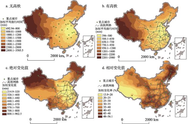
Fig. 2 The spatial pattern of location indicator analysis between without and with HSR scenarios in 2020图2 2020年高铁通车前后全国陆路加权旅行时间空间格局分析图 |
Tab. 2 The variation for selected accessibility indicators between without and with HSR scenarios in 2020表2 2020年高铁通车前后全国县级以上城市可达性值的变化 |
| 指标 | 无高铁 | 有高铁 | 变化率(%) | |||||||||
|---|---|---|---|---|---|---|---|---|---|---|---|---|
| 最小值 | 平均值 | 最大值 | 变异系数 | 最小值 | 平均值 | 最大值 | 变异系数 | 平均值 | 变异系数 | |||
| 加权平均旅行 时间(min) | 692.86 | 1188.58 | 3585.5 | 0.44 | 395.97 | 723.95 | 2979.55 | 0.56 | 39.0 | 28.0 | ||
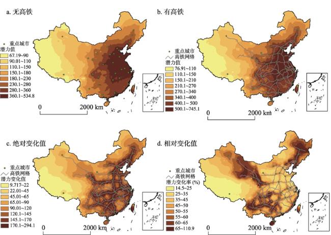
| 潜力可达性 | 67.19 | 300.42 | 536.66 | 0.37 | 76.9 | 442.9 | 745.1 | 0.35 | 47.4 | 6.4 | ||
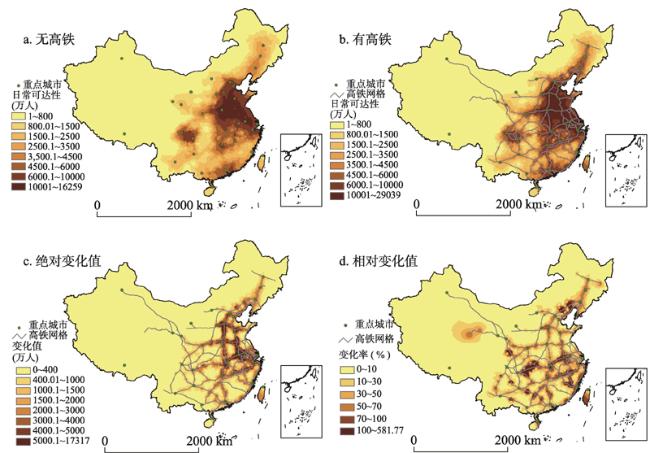
| 日常可达性(万人) | 1 | 4011.79 | 16262.13 | 0.93 | 1 | 5416.24 | 29040.95 | 1 | 35.0 | 7.30 | ||
Fig. 3 Daily accessibility indicator spatialpattern analysis maps between without and with HSR scenarios in 2020图3 2020年高铁通车前后全国陆路日常可达性空间格局分析图 |
Tab. 3 Daily accessibility indicators for the major cities without and with HSR scenarios in 2020表3 2020年高铁通车前后重点城市4 h可达性变化 |
| 城市 | 无高铁 (万人) | 有高铁 (万人) | 变化值 (万人) | 变化率(%) | 城市 | 无高铁 (万人) | 有高铁 (万人) | 变化值 (万人) | 变化率(%) |
|---|---|---|---|---|---|---|---|---|---|
| 拉萨 | 90.1 | 90.1 | 0 | 0 | 太原 | 4560.79 | 7345.22 | 2784.43 | 61.1 |
| 台北 | 260 | 260 | 0 | 0 | 天津 | 7401.7 | 12605.96 | 5204.26 | 70.3 |
| 乌鲁木齐 | 601.48 | 601.48 | 0 | 0 | 杭州 | 8524.21 | 14749.81 | 6225.6 | 73.0 |
| 银川 | 805.42 | 805.42 | 0 | 0 | 沈阳 | 3886.79 | 6783.38 | 2896.59 | 74.5 |
| 呼和浩特 | 1404.78 | 1504.98 | 100.2 | 7.1 | 长沙 | 6420.22 | 11366.09 | 4945.87 | 77.0 |
| 西宁 | 1210.57 | 1312.17 | 101.6 | 8.4 | 郑州 | 12308.11 | 22348.72 | 10040.61 | 81.6 |
| 昆明 | 2466.44 | 2883.64 | 417.2 | 16.9 | 济南 | 11367.45 | 20694.12 | 9326.67 | 82.0 |
| 重庆 | 6567.07 | 7957.37 | 1390.3 | 21.2 | 西安 | 3914.57 | 7184.1 | 3269.53 | 83.5 |
| 贵阳 | 2893.5 | 3717.79 | 824.29 | 28.5 | 南京 | 10065.76 | 18593.57 | 8527.81 | 84.7 |
| 兰州 | 2243.22 | 2925.61 | 682.39 | 30.4 | 长春 | 3368.6 | 6301.59 | 2932.99 | 87.1 |
| 南宁 | 2818.51 | 3800.51 | 982 | 34.8 | 石家庄 | 9343.28 | 18159.98 | 8816.7 | 94.4 |
| 成都 | 5521.04 | 7617.87 | 2096.83 | 38.0 | 海口 | 1146.33 | 2427.83 | 1281.5 | 111.8 |
| 北京 | 6903.7 | 10392.9 | 3489.24 | 50.5 | 福州 | 2892.3 | 6500.44 | 3608.14 | 124.7 |
| 哈尔滨 | 3192.2 | 4961.47 | 1769.27 | 55.4 | 南昌 | 5026.02 | 11976.13 | 6950.11 | 138.3 |
| 广州 | 5889.66 | 9276.85 | 3387.19 | 57.5 | 合肥 | 8885.66 | 22672.54 | 13786.88 | 155.2 |
| 上海 | 7078.98 | 11333 | 4254.03 | 60.1 | 武汉 | 5067.93 | 16595.1 | 11527.17 | 227.5 |
Fig. 4 Potential indicator spatial pattern analysis between without and with HSR scenarios in 2020图4 2020年高铁通车前后全国陆路潜力可达性的空间格局分析图 |
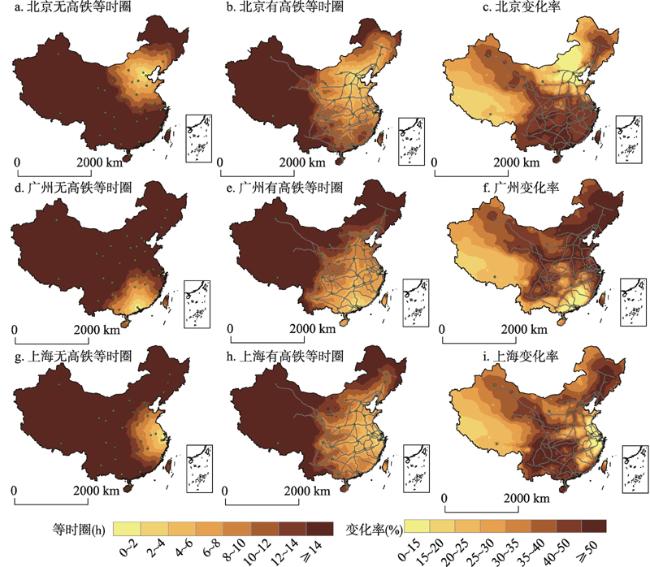
Fig. 5 Primate cities' isochrones spatial pattern in three urban agglomerations图5 三大城市群首位城市等时圈空间格局分析 |
Tab. 4 Primate cities' isochrones areal analysis in three urban agglomerations表4 三大城市群的首位城市等时间圈分析 |
| 城市 | 通车前各时间圈(h) | 通车后各时间圈(h) | |||||||||
|---|---|---|---|---|---|---|---|---|---|---|---|
| 0~2 | 2~4 | 4~6 | 6~8 | 8~10 | 0~2 | 2~4 | 4~6 | 6~8 | 8~10 | ||
| 北京 | 可达面积(km2) | 17657 | 117318 | 219118 | 354666 | 518204 | 17749 | 181451 | 659819 | 973109 | 1181971 |
| 上海 | 12285 | 76452 | 157182 | 183693 | 300616 | 12612 | 150326 | 530218 | 814470 | 1079559 | |
| 广州 | 24812 | 99406 | 135002 | 176595 | 275532 | 25099 | 145877 | 435428 | 908679 | 840771 | |
| 北京 | 可达人口(万人) | 1818.4 | 5085.3 | 6843.07 | 10462.98 | 16354.44 | 1818.4 | 8574.54 | 28006.22 | 32524.16 | 24664.37 |
| 上海 | 2313.78 | 4765.2 | 7617.96 | 9916.52 | 15622.16 | 2313.78 | 9019.23 | 28491.74 | 39974.54 | 27205.95 | |
| 广州 | 2131.37 | 3758.29 | 5646.86 | 6145.45 | 8143.13 | 2131.37 | 7145.48 | 16620.5 | 33503.23 | 40989.09 | |
| 北京 | 可达GDP(亿元) | 15418.64 | 23049.72 | 25642.50 | 33282.29 | 55128.90 | 15418.64 | 34907.14 | 96663.95 | 135882.80 | 79469.03 |
| 上海 | 29063.45 | 35950.04 | 26760.66 | 20058.91 | 44554.45 | 29063.45 | 53401.03 | 85281.30 | 146229.29 | 71374.75 | |
| 广州 | 25270.65 | 16559.16 | 9636.42 | 16223.39 | 21677.72 | 25270.65 | 26202.59 | 45966.79 | 118405.57 | 125155.97 | |
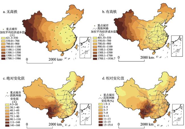
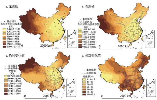
Tab. 5 Weighted average travel cost indicators changes for two different income groups between without and with HSR scenarios in 2020表5 2020年高铁通车前后不同收入群体加权平均经济可达性变化 |
| 指标 | 无高铁 | 有高铁 | 变化率 | |||||||||
|---|---|---|---|---|---|---|---|---|---|---|---|---|
| 最小值(元) | 平均值 (元) | 最大值 (元) | 变异系数 | 最小值 (元) | 平均值(元) | 最大值(元) | 变异系数 | 平均值(%) | 变异系数 | |||
| 平均工资经济可达性 | 421.2 | 704.3 | 1986 | 0.423 | 401.32 | 657.50 | 1936.68 | 0.429 | 6.45 | 1.4 | ||
| 高收入经济可达性 | 2492.97 | 4261.6 | 12819.32 | 0.436 | 1669.61 | 2932.694 | 10886.96 | 0.511 | 31.1 | 17.1 | ||
Fig. 6 Weighted average travel cost indicators spatial pattern for general income travelers图6 普通出行者经济成本可达性空间格局 |
Fig. 7 Weighted average travel cost indicators spatial pattern for high income travelers图7 高收入出行者经济成本可达性空间格局 |
The authors have declared that no competing interests exist.
| [1] |
|
| [2] |
|
| [3] |
|
| [4] |
|
| [5] |
|
| [6] |
|
| [7] |
|
| [8] |
[
|
| [9] |
[
|
| [10] |
[
|
| [11] |
|
| [12] |
[
|
| [13] |
[
|
| [14] |
|
| [15] |
[
|
| [16] |
[
|
| [17] |
[
|
| [18] |
[
|
| [19] |
|
| [20] |
|
| [21] |
|
| [22] |
|
/
| 〈 |
|
〉 |