
基于粒子群算法的大城市近郊区景观格局优化研究——以成都市龙泉驿区为例
作者简介:欧定华(1984- ),男,四川宜宾人,博士研究生,主要从事景观生态规划与设计、土地利用规划与管理、“3S”技术应用研究。E-mail:357881550@qq.com
收稿日期: 2016-07-14
要求修回日期: 2016-12-05
网络出版日期: 2017-03-20
基金资助
国家自然科学基金项目(31270498)
四川省学术和技术带头人培养经费(2014)
四川农业大学双支计划项目(2015)
Landscape pattern optimization in peri-urban areas based on the particle swarm optimization method: A case study in Longquanyi District of Chengdu
Received date: 2016-07-14
Request revised date: 2016-12-05
Online published: 2017-03-20
Copyright
景观格局优化是实现区域生态安全的重要途径。以成都市龙泉驿为研究区,在景观适宜性评价、景观数量优化基础上,构建PSO景观格局空间优化模型与求解算法,对经济发展、生态保护、统筹兼顾情景景观空间布局进行优化。结果表明:基于PSO的景观格局空间优化模型与算法能利用粒子位置模拟景观分布进行空间格局优化,实现了数量与空间优化的有机耦合,是景观格局优化的有效方法。目标年,经济发展情景优势景观为城乡人居及工矿、果园,景观格局呈现出西部坝区以城乡人居及工矿、农田为主,东部山区以果园为主的分布特征;生态保护情景优势景观为森林、城乡人居及工矿,景观格局呈现出西部坝区以城乡人居及工矿、果园、农田为主,东部山区以森林为主的分布特征;统筹兼顾情景优势景观为森林、城乡人居及工矿和果园,景观格局呈现出西部坝区以城乡人居及工矿、农田为主,东部山区以森林、果园为主的分布特征。统筹兼顾情景方案未来潜在可能性最大,其经济、生态、综合效益均得以优化提升,是目标年研究区最佳景观格局空间布局方案。
欧定华 , 夏建国 . 基于粒子群算法的大城市近郊区景观格局优化研究——以成都市龙泉驿区为例[J]. 地理研究, 2017 , 36(3) : 553 -572 . DOI: 10.11821/dlyj201703013
Landscape pattern optimization is one of the important ways in achieving regional ecological security. In order to optimize landscape spatial layout of economic development, ecological protection and overall consideration scenario, a case study was carried out in Longquanyi District of Chengdu based on landscape suitability assessment and landscape quantity optimization. The method of particle swarm optimization (PSO) was used to establish landscape pattern spatial optimization model and algorithm. The results showed that, the landscape pattern spatial optimization model and algorithm based on PSO was the effective method of landscape pattern optimization. The model and algorithm could efficiently simulate landscape distribution by using particle space positions, conduct spatial pattern optimization, and realize united coupling of quantity structure and spatial distribution optimization. The dominant landscapes in economic development scenario were orchard, urban-rural residential and industrial-mining area in a target year. The landscape pattern showed that farmland, urban-rural residential and industrial-mining area dominated the western flatland region, while eastern mountainous area was mainly dominated by orchard. The dominant landscapes in ecological protection scenario were forest, urban-rural residential and industrial-mining area. The landscape pattern showed that the western flatland region was mainly dominated by farmland, orchard, urban-rural residential and industrial-mining area, while the eastern mountainous area was dominated by forest. The dominant landscapes in overall consideration scenario were forest, orchard, urban-rural residential and industrial-mining area. The landscape pattern showed that farmland, urban-rural residential and industrial-mining area dominated the western flatland region, while eastern mountainous area was dominated by forest and orchard. Compared with other scenarios, the overall consideration scenario could be the largest potential possibility in the future, since the economic, ecological and comprehensive benefits here would be the most optimized and promoted, implying the best spatial layout scheme for landscape pattern in the study area in the target year.
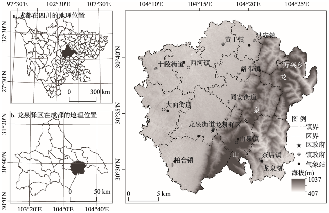
Fig. 1 Geographical location of the study area图1 研究区地理位置 |
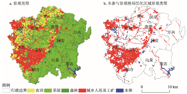
Fig. 2 Landscape map of the study area and landscape map outside of range for landscape pattern optimization图2 研究区景观类型图与未参与景观格局优化区域景观类型图 |
Tab. 1 Index system of landscape suitability assessment表1 景观适宜性评价指标体系 |
| 一级指标 | 二级指标 | 数据来源与说明 | 空间化方法 |
|---|---|---|---|
| 自然因子 | 高程 | ASTER GDEM V2数据,分辨率30 m | 利用ArcGIS 10.0裁剪得到研究区高程数据,并将栅格分辨率重采样为60 m |
| 坡度 | 同高程指标 | 应用ArcGIS 10.0空间分析工具基于高程数据计算坡度、坡向,分辨率60 m | |
| 坡向 | 同高程指标 | ||
| 地势起伏度 | 同高程指标 | 应用ArcGIS 10.0空间分析工具基于高程数据按公式[25]计算地势起伏度,分辨率60 m | |
| 多年平均降雨量 | 2004-2014年龙泉驿9个自动气象观测站(图1)监测的降雨、气温数据(来自区气象局) | 应用ArcGIS 10.0规则样条函数空间插值法得到降雨、气温、土壤有机质含量空间分布数据,分辨率60 m | |
| 多年平均气温 | |||
| 土壤有机质含量 | 龙泉驿区测土配方施肥项目监测的有机质含量数据(来自区农林局农技中心) | ||
| 邻域因子 | 到城市中心最近距离 | 2014年景观类型图 | 首先用ArcGIS 10.0矢量工具绘制主城区范围,然后用Feature To Point工具获取主城区图斑几何中心点作为城市中心,最后利用欧氏距离分析工具求得景观类型图各栅格点到城市中心的最近距离,分辨率60 m |
| 到建制镇中心最近距离 | 2014年景观类型图和各街镇乡行政中心矢量图(来自龙泉驿区第二次全国土地调查成果) | 利用ArcGIS 10.0欧氏距离分析工具求得景观类型图各栅格点到街镇乡行政中心的最近距离,分辨率60 m | |
| 到主要道路最近距离 | 2014年景观类型图 | 首先用ArcGIS 10.0从景观类型图中提取高速公路、交通干道等主要道路数据,然后用欧氏距离分析工具求得景观类型图各栅格点到主要道路的最近距离,分辨率60 m | |
| 到主要水域最近距离 | 首先用ArcGIS 10.0从景观类型图中提取水渠、水库、坑塘等主要水域数据,然后用欧氏距离分析工具求得景观类型图各栅格点到主要水域的最近距离,分辨率60 m | ||
| 社会经济 因子 | 人口密度 | 各街镇乡行政区矢量数据(来自龙泉驿区第二次全国土地调查成果),龙泉驿统计年鉴(2000-2012年)、成都统计信息网(http://www.chdstats.gov.cn)以及龙泉驿区统计局、各街镇乡统计资料 | 首先统计12个街镇乡人口密度、人均地区生产总值,然后用ArcGIS10.0将其链接到行政区矢量数据属性表对应行记录并通过矢栅转化得到人口密度、人均地区生产总值空间数据,分辨率60 m |
| 人均地区生产总值 |
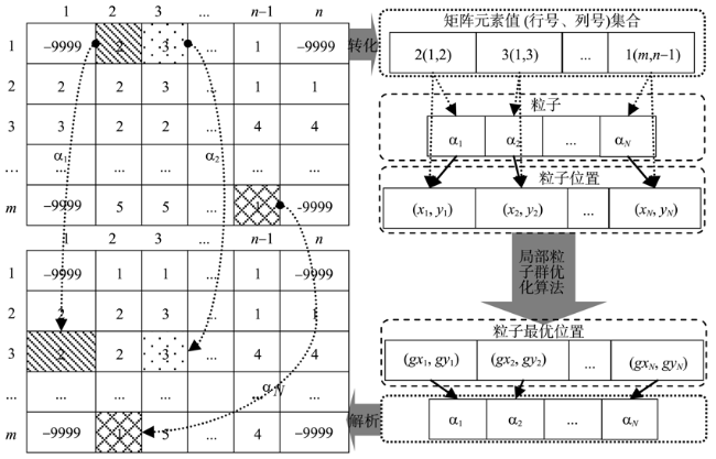
Fig. 3 Schematic diagram of landscape pattern spatial optimization model based on PSO图3 PSO景观格局空间优化模型示意图 |
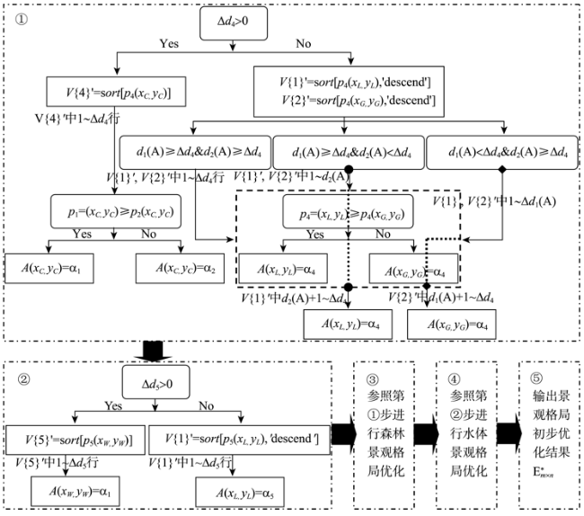
Fig.4 Flow chart of particles initialization图4 粒子初始化流程图 |
Tab. 2 Regression coefficients and significant test results of binary Logistic models表2 Logistic模型回归系数及显著性检验结果 |
| 评价指标 | 农田 | 果园 | 森林 | 城乡人居及工矿 | 水体 | |||||||||
|---|---|---|---|---|---|---|---|---|---|---|---|---|---|---|
| 回归系数 | 显著性 | 回归系数 | 显著性 | 回归系数 | 显著性 | 回归系数 | 显著性 | 回归系数 | 显著性 | |||||
| 高程 | -6.37E-03 | 0.0000 | 2.34E-03 | 0.0000 | -1.49E-03 | 0.0066 | - | 0.0630 | -8.56E-03 | 0.0000 | ||||
| 坡度 | - | 0.0470 | - | 0.9150 | - | 0.9450 | - | 0.4110 | - | 0.8970 | ||||
| 坡向 | - | 0.0570 | - | 0.0450 | - | 0.0230 | — | 0.3100 | — | 0.0670 | ||||
| 地势起伏度 | -0.0119 | 0.0000 | 1.17E-03 | 0.0129 | 2.69E-03 | 0.0004 | -2.86E-03 | 0.0003 | 4.83E-03 | 0.0002 | ||||
| 到城市中心最近距离 | 6.99E-05 | 0.0000 | 9.93E-05 | 0.0000 | 1.38E-04 | 0.0000 | -1.90E-04 | 0.0000 | - | 0.0960 | ||||
| 到建制镇中心最近距离 | 2.72E-04 | 0.0000 | - | 0.7540 | - | 0.1220 | -1.08E-04 | 0.0000 | -1.57E-04 | 0.0031 | ||||
| 到主要道路最近距离 | -9.97E-05 | 0.0051 | - | 0.7550 | -1.63E-04 | 0.0000 | - | 0.1400 | - | 0.2680 | ||||
| 到主要水域最近距离 | - | 0.0160 | - | 0.1230 | -1.59E-04 | 0.0005 | 3.45E-04 | 0.0000 | -6.65E-04 | 0.0000 | ||||
| 多年平均降雨量 | -3.19E-03 | 0.0000 | 6.44E-03 | 0.0000 | 7.14E-03 | 0.0000 | -0.0110 | 0.0000 | - | 0.0820 | ||||
| 多年平均气温 | - | 0.1660 | - | 0.0400 | -1.21 | 0.0000 | 0.3720 | 0.0000 | - | 0.2650 | ||||
| 土壤有机质含量 | 0.0221 | 0.0000 | - | 0.1060 | - | 0.5790 | -0.0308 | 0.0000 | - | 0.7210 | ||||
| 人口密度 | - | 0.2770 | -1.19E-04 | 0.0003 | - | 0.3910 | - | 0.0780 | - | 0.6480 | ||||
| 人均地区生产总值 | -0.0172 | 0.0001 | 0.0425 | 0.0000 | 0.0442 | 0.0000 | -0.0604 | 0.0000 | - | 0.5980 | ||||
| 常量 | 2.49 | 0.0001 | -7.29 | 0.0000 | 10.6 | 0.0000 | 3.82 | 0.0015 | 1.33 | 0.0016 | ||||
| ROC | 0.8040 | 0.7125 | 0.7892 | 0.7858 | 0.7000 | |||||||||
Tab. 3 Optimization results of landscape areas for each scenario in target year (hm2)表3 目标年各情景景观面积优化结果(hm2) |
| 目标年 | 规划情景 | 农田 | 果园 | 森林 | 城乡人居及工矿 | 水体 |
|---|---|---|---|---|---|---|
| 2021年 | 经济发展 | 7235.00 | 21803.00 | 5167.00 | 19754.00 | 1610.00 |
| 生态保护 | 7235.00 | 7380.75 | 23136.25 | 16207.00 | 1610.00 | |
| 统筹兼顾 | 7235.00 | 16231.31 | 10738.69 | 19754.00 | 1610.00 | |
| 2028年 | 经济发展 | 7901.00 | 19305.00 | 5167.00 | 21586.00 | 1610.00 |
| 生态保护 | 7901.00 | 5216.00 | 24635.00 | 16207.00 | 1610.00 | |
| 统筹兼顾 | 7901.00 | 5216.00 | 19256.00 | 21586.00 | 1610.00 | |
| 基期年(2014年) | 景观格局现状 | 6723.00 | 25862.00 | 5167.00 | 16207.00 | 1610.00 |
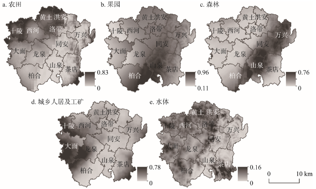
Fig. 5 Suitability assessment results of landscapes for farmland, orchard, forest, urban-rural residential as well as industrial-mining and water body图5 农田、果园、森林、城乡人居及工矿、水体景观适宜性评价图 |
Tab. 4 Solving results of PSO landscape pattern spatial optimization model for each scenario in target year表4 目标年各情景PSO景观格局空间优化模型求解结果 |
| 目标年 | 规划情景 | 农田(栅格) | 果园(栅格) | 森林(栅格) | 城乡人居及工矿(栅格) | 水体(栅格) |
|---|---|---|---|---|---|---|
| 2021年 | 经济发展 | 19870(0.98%) | 60677(0.34%) | 14600(1.88%) | 54541(0.45%) | 4435(0.67%) |
| 生态保护 | 19796(1.35%) | 20950(2.34%) | 64261(0.14%) | 44664(0.64%) | 4452(0.29%) | |
| 统筹兼顾 | 19890(0.88%) | 45121(0.23%) | 30165(1.28%) | 54539(0.46%) | 4408(1.28%) | |
| 2028年 | 经济发展 | 21754(0.73%) | 53271(0.51%) | 14829(3.47%) | 59825(0.08%) | 4444(0.47%) |
| 生态保护 | 21810(0.47%) | 14734(1.85%) | 68246(0.12%) | 44905(0.10%) | 4428(0.83%) | |
| 统筹兼顾 | 21840(0.34%) | 14533(0.46%) | 53570(0.31%) | 59705(0.28%) | 4475(0.22%) | |
| 基期年(2014) | 景观格局现状 | 22136 | 82917 | 14268 | 30439 | 4363 |
注:表中圆括弧内数据为景观格局空间优化结果与数量优化结果的相对误差,栅格大小为60 m×60 m。 |
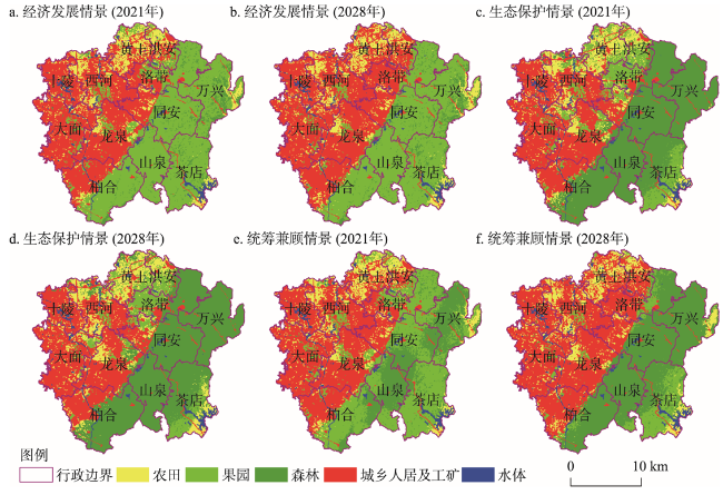
Fig. 6 Result maps of landscape pattern spatial optimization for each scenario in target year图6 目标年各情景景观格局空间优化结果图 |
The authors have declared that no competing interests exist.
| [1] |
[
|
| [2] |
[
|
| [3] |
[
|
| [4] |
|
| [5] |
|
| [6] |
|
| [7] |
[
|
| [8] |
[
|
| [9] |
[
|
| [10] |
[
|
| [11] |
[
|
| [12] |
|
| [13] |
[
|
| [14] |
[
|
| [15] |
[
|
| [16] |
[
|
| [17] |
[
|
| [18] |
[
|
| [19] |
[
|
| [20] |
[
|
| [21] |
[
|
| [22] |
[
|
| [23] |
[
|
| [24] |
[
|
| [25] |
[
|
| [26] |
|
| [27] |
[
|
| [28] |
[
|
| [29] |
[
|
| [30] |
[
|
| [31] |
[
|
| [32] |
[
|
| [33] |
[
|
| [34] |
[
|
| [35] |
[
|
/
| 〈 |
|
〉 |